Graph Convolution Network (GCN) and Graph Attention Network (GAT)

• Introduction to GCN
• GraphSAGE
• Defferrard, Michaël, Xavier Bresson, and Pierre Vandergheynst. "Convolutional neural networks on graphs with fast localized spectral filtering." Advances in neural information processing systems 29 (2016).
• Kipf, Thomas N., and Max Welling. "Semi-supervised classification with graph convolutional networks." International Conference on Learning Representations (2017).
• Hamilton, Will, Zhitao Ying, and Jure Leskovec. "Inductive representation learning on large graphs." Advances in neural information processing systems 30 (2017).
• Wu, Felix, Amauri Souza, Tianyi Zhang, Christopher Fifty, Tao Yu, and Kilian Weinberger. "Simplifying graph convolutional networks." In International conference on machine learning, pp. 6861-6871. PMLR, 2019.
• Veličković, Petar, Guillem Cucurull, Arantxa Casanova, Adriana Romero, Pietro Lio, and Yoshua Bengio. "Graph attention networks." International Conference on Learning Representations (2018).

1. Laplacian Matrix on Graph

The Laplacian matrix of a $n$-vertex graph $\mathcal{G}$ is defined as $$L = D - W,$$ where $W \in \mathbb{R}^{n \times n}$ is the adjacent matrix with weights $W_{ij}$ and $D = \mathrm{diag}(D_i) \in \mathbb{R}^{n \times n}, D_i = \sum_{j}W_{ij}$ is the degree matrix. The normalized Laplacian matrix is defined as $$L_{N}=D^{-1 / 2}(D-W) D^{-1 / 2} = I_n - D^{-1 / 2} W D^{-1 / 2}.$$ The Laplace operator is defined as $$\Delta f=\sum_{i=1}^{n} \frac{\partial^{2} f}{\partial x_{i}^{2}},$$ In $1$-dimensional space, we have $$\begin{aligned} \frac{\partial^{2} f}{\partial x_{i}^{2}} =f^{\prime \prime}(x) & \approx f^{\prime}(x)-f^{\prime}(x-1) \\ & \approx f(x+1)-f(x)-(f(x)-f(x-1)) \\ &=f(x+1)+f(x-1))-2 f(x). \end{aligned}$$ Similarly, if we consider a $n$-vertex graph $\mathcal{G}$ and a function $\mathbf{f}$ on it, $$\mathbf{f} = (f_1, \ldots, f_n),$$ where $f_i$ is the function value of the $i$-th vertex in the graph. Then the Laplacian operation on this function $\mathbf{f}$ on graph $\mathcal{G}$ should be $$\begin{aligned} \Delta f_{i} =\sum_{j \in N_{i}} \frac{\partial f_{i}}{\partial j^{2}} & \approx \sum_{j} W_{i j}\left(f_{i}-f_{j}\right) \\ &=\sum_{j} W_{i j}\left(f_{i}-f_{j}\right) \\ &=\left(\sum_{j} W_{i j}\right) f_{i}-\sum_{j} W_{i j} f_{j} \\ &=D_{i} f_{i}-\sum_{j} W_{i j} f_{j}. \end{aligned}$$ In a vector form, we can recover the definition of Laplacian matrix on graph $\mathcal{G}$, $$\Delta \mathbf{f} = (D - W) \mathbf{f} = L \mathbf{f}.$$ For an undirected graph, the Laplacian matrix is a real symmetric matrix and therefore we have the spectral decomposition $$L = U \Lambda U^\top, \;\; \Lambda = \mathrm{diag}(\lambda_1, \ldots, \lambda_n).$$ There are also some properties for Laplacian matrix $L$,

• There is at least one eigenvalue 0.
• All the eigenvalues are non-negative. For normalized Laplacian matrix, all the eigenvalues are between 0 and 2, and the summation is $n$.
• If there are $k$ eigenvalues with value 0, then there are $k$ mutually unconnected sub-graphs within the graph.

2. Fourier Transformer

Recall Fourier transformer of function $f(\cdot)$, $$\mathcal{F}_{T}(\omega)=\int_{-\infty}^{+\infty} f(t) e^{-i \omega t} d t,$$ where $\{e^{-iwt}\}$ is a set of orthogonal basis. We also have the inverse Fourier transformer, $$f(t)=\frac{1}{2 \pi} \int_{-\infty}^{+\infty} \mathcal{F}_{T}(\omega) e^{i \omega t} d \omega.$$

For the basis function $\{e^{-iwt}\}$, notice that it is the eigenfunction for Laplacian operator $\Delta$, $$\Delta e^{-i \omega t}=\nabla^{2} e^{-i \omega t}=\frac{d e^{-i \omega t}}{d t^{2}}=-\omega^{2} e^{-i \omega t}.$$ Similarly, the eigenvectors $U = [\mathbf{u}_1, \ldots, \mathbf{u}_n]$ of graph Laplacian matrix should also be the basis for the Fourier transformer on the graph $\mathcal{G}$, i.e., $$\mathcal{F}_T\left(\lambda_{k}\right) \triangleq \hat{f}_{k}= \langle \mathbf{f}, \mathbf{u}_k \rangle = \sum_{i=1}^{n} f_i \mathbf{u}_{k}(i).$$ Therefore, $$\hat{\mathbf{f}} = U^\top \mathbf{f}.$$ Similarly, we have the inverse Fourier transformer on graph $\mathcal{G}$, $$\mathbf{f} = U \hat{\mathbf{f}} = U U^\top \mathbf{f}.$$

3. Convolution on Graphs

Denote the continuous convolution for two functions $f, g$, $$(f * g)(t) \stackrel{\text { def }}{=} \int_{\mathbb{R}^{n}} f(\tau) g(t-\tau) d \tau,$$ as well as the discrete convolution, $$(f * g)(n)=\sum_{m=-\infty}^{\infty} f(m) g(n-m)=\sum_{m=-\infty}^{\infty} f(n-m) g(m).$$ Recall the property for convolution and Fourier transformer, $$\mathcal{F}\{f * g\}=\mathcal{F}\{f\} \cdot \mathcal{F}\{g\}.$$ Therefore, $$f * g=\mathcal{F}^{-1} \left(\mathcal{F}\{f\} \cdot \mathcal{F}\{g\} \right).$$ For convolution operations on graph $\mathcal{G}$, similarly, we have $$(\mathbf{f} * \mathbf{g})_{\mathcal{G}} =\mathcal{F}^{-1}[\mathcal{F}\{\mathbf{f}\} \cdot \mathcal{F}\{\mathbf{g}\}] =\mathcal{F}^{-1}\left[U^{T} \mathbf{f} \cdot \hat{\mathbf{g}}\right] = \mathcal{F}^{-1}\left[\mathrm{diag}(\hat{g}_1, \ldots, \hat{g}_n) U^{T} \mathbf{f} \right].$$ If we parameterize $\hat{\mathbf{g}}$ directly by trainable parameters $\theta_1, \ldots, \theta_n$, $$(\mathbf{f} * \mathbf{g})_{\mathcal{G}} = U \mathrm{diag}(\theta_1, \ldots, \theta_n) U^{T} \mathbf{f}.$$ This is the convolution filter on graphs.

4. Fast Localized Spectral Filtering

• Defferrard, Michaël, Xavier Bresson, and Pierre Vandergheynst. "Convolutional neural networks on graphs with fast localized spectral filtering." Advances in neural information processing systems 29 (2016).

Recall that in the above graph convolution, $\hat{\mathbf{g}}$ is a vector depending on the eigenvalues of the Laplacian matrix $L$, we can rewrite it as $$\hat{\mathbf{g}} = g_\theta(\Lambda),$$ and the graph convolution is then $$\mathbf{y} = U g_\theta(\Lambda) U^{T} \mathbf{x}.$$ Notice that it can also be seen as a signal $\mathbf{x}$ filtered by $g_\theta$ as, $$\mathbf{y} = g_\theta(L) \mathbf{x} = g_\theta(U \Lambda U^\top) \mathbf{x} = U g_\theta(\Lambda) U^{T} \mathbf{x}.$$ The parameterization in the previous section can be seen as a non-parametric filter, i.e., $$g_\theta(\Lambda) = \mathrm{diag}(\theta_1, \ldots, \theta_n).$$ There are however two limitations with non-parametric filters:

• they are not localized in space
• their learning complexity is in $\mathcal{O}(n)$, the dimensionality of the graph.

These issues can be overcome with the use of a polynomial filter, $$g_\theta(\Lambda) = \sum_{k=0}^{K-1} \theta_{k} \Lambda^{k}.$$ Under the polynomial filter, the convolution is given by $$\mathbf{y} = U g_\theta(\Lambda) U^\top \mathbf{x} = \left(\sum_{k=0}^{K-1} \theta_{k} L^{k}\right) \mathbf{x}.$$ Notice that $d_{\mathcal{G}}(i, j)>K$ implies $\left(L^{K}\right)_{i, j}=0$, where $d_{\mathcal{G}}$ is the shortest path distance between $i$ and $j$. Consequently, spectral filters represented by $K^{\text {th }}$ order polynomials of the Laplacian matrix are exactly $K$-localized. Besides, their learning complexity is $\mathcal{O}(K)$, the support size of the filter, and thus the same complexity as classical CNNs.

However, the matrix computation of $U$ matrix part still involves the $\mathcal{O}(n^2)$ computation complexity. Recall that the Chebyshev polynomial $T_{k}(x)$ of order $k$ may be computed by the stable recurrence relation $$T_{k}(x)=2 x T_{k-1}(x)-T_{k-2}(x),$$ with $T_{0}=1$ and $T_{1}=x$. These polynomials form an orthogonal basis for $L^{2}\left([-1,1], d y / \sqrt{1-y^{2}}\right)$, the Hilbert space of square integrable functions with respect to the measure $d y / \sqrt{1-y^{2}}$. A filter can thus be parametrized as the truncated expansion, $$g_{\theta}(\Lambda)=\sum_{k=0}^{K-1} \theta_{k} T_{k}(\widetilde{\Lambda}),$$ where $$\widetilde{\Lambda}=2 \Lambda / \lambda_{\max }-I_{n}$$ is the normalized diagonal matrix with scaled eigenvalues that lie in $[-1,1]$. The convolution operation is therefore, $$\mathbf{y} = \sum_{k=0}^{K-1} \theta_{k} T_{k}(\widetilde{L}) \mathbf{x}.$$ Here $\widetilde{L}=2 L / \lambda_{\max }-I_{n}$. Denoting $\bar{\mathbf{x}}_{k}=T_{k}(\widetilde{L}) \mathbf{x} \in \mathbb{R}^{n}$, we can use the recurrence relation to compute $\bar{\mathbf{x}}_{k}=2 \widetilde{L} \bar{\mathbf{x}}_{k-1}-\bar{\mathbf{x}}_{k-2}$ with $\bar{\mathbf{x}}_{0}=\mathbf{x}$ and $\bar{\mathbf{x}}_{1}=\widetilde{L} \mathbf{x}$. The entire filtering operation then costs $\mathcal{O}(K|\mathcal{E}|)$ operations, where $|\mathcal{E}|$ is the number of edges in the graph $\mathcal{G}$.

5. Fast Approximate Convolutions on Graphs

• Kipf, Thomas N., and Max Welling. "Semi-supervised classification with graph convolutional networks." International Conference on Learning Representations (2017).

Recall that in the previous section, we have the convolution operation on vector $\mathbf{x}$ of a graph $\mathcal{G}$ using Chebyshev polynomials, $$\mathbf{y} = \sum_{k=0}^{K-1} \theta_{k} T_{k}(\widetilde{L}) \mathbf{x}.$$ If we consider the simple case of $K=2$ and consider the normalized Laplacian matrix $L_N$, and approximate $\lambda_{\max}=2$, which is the eigenvalue upper bound for $L_N$, we have $$\mathbf{y} = \sum_{k=0}^{1} \theta_{k} T_{k}(\widetilde{L}_N) \mathbf{x} = \theta_{0} \mathbf{x}+\theta_{1}\left(L_N-I_{n}\right) \mathbf{x}=\theta_{0} \mathbf{x}-\theta_{1} D^{-\frac{1}{2}} W D^{-\frac{1}{2}} \mathbf{x}.$$ In practice, it can be beneficial to constrain the number of parameters further to address overfitting and to minimize the number of operations (such as matrix multiplications) per layer. This leaves us with the following expression using $\theta = \theta_0 = - \theta_1$, $$\mathbf{y} = \theta \mathbf{x} + \theta D^{-\frac{1}{2}} W D^{-\frac{1}{2}} \mathbf{x} = \theta \left(I_n + D^{-\frac{1}{2}} W D^{-\frac{1}{2}} \right) \mathbf{x}.$$ Note that $I_{n}+D^{-\frac{1}{2}} W D^{-\frac{1}{2}}$ now has eigenvalues in the range $[0,2]$. Repeated application of this operator can therefore lead to numerical instabilities and exploding/vanishing gradients when used in a deep neural network model.

To alleviate this problem, we introduce the following renormalization trick: $$I_{n}+D^{-\frac{1}{2}} W D^{-\frac{1}{2}} \rightarrow \widetilde{D}^{-\frac{1}{2}} \widetilde{W} \widetilde{D}^{-\frac{1}{2}},$$ with $\widetilde{W}=W+I_{N}$ and $\widetilde{D}_{i i}=\sum_{j} \widetilde{W}_{i j}$.

We can generalize this definition to a signal $X \in \mathbb{R}^{N \times C}$ with $C$ input channels (i.e. a $C$-dimensional feature vector for every node) and $F$ filters or feature maps as follows, $$Y=\tilde{D}^{-\frac{1}{2}} \tilde{W} \tilde{D}^{-\frac{1}{2}} X \Theta,$$ where $\Theta \in \mathbb{R}^{C \times F}$ is now a matrix of filter parameters and $Y \in \mathbb{R}^{N \times F}$ is the convolved signal matrix. This filtering operation has complexity $\mathcal{O}(|\mathcal{E}| F C)$, as $\tilde{W} X$ can be efficiently implemented as a product of a sparse matrix with a dense matrix.

6. Simple GCN

• Wu, Felix, Amauri Souza, Tianyi Zhang, Christopher Fifty, Tao Yu, and Kilian Weinberger. "Simplifying graph convolutional networks." In International conference on machine learning, pp. 6861-6871. PMLR, 2019.

From Kipf and Welling (2017) above, for a input $X^{(t)} \in \mathbb{R}^{N \times C}$ with $C$ input channels (i.e. a $C$-dimensional feature vector for every node) and $F$ filters or feature maps as follows, $$X^{(t+1)}= \sigma\left(S X^{(t)} \Theta \right), \; \; S = \tilde{D}^{-\frac{1}{2}} \tilde{W} \tilde{D}^{-\frac{1}{2}}.$$ where $\Theta \in \mathbb{R}^{C \times F}$ is now a matrix of filter parameters, $\sigma$ is the non-liner activation function and $X^{(t+1)} \in \mathbb{R}^{N \times F}$ is the convolved signal matrix. For a $K$-depth network, we will repeat the above procedure $K$ times.

This paper hypothesizes that the nonlinearity between GCN layers is not critical - but that the majority of the benefit arises from the local averaging. The resulting model is linear, but still has the same increased “receptive field” of a $K$-layer GCN, i.e., $$Y =\operatorname{softmax}\left(S \ldots S S X \Theta^{(1)} \Theta^{(2)} \ldots \Theta^{(K)}\right) = \operatorname{softmax} \left(S^K X \Theta\right).$$ Under this network, the authors obtain a comparable experiment results with the previous structure, and the computation cost / the number of parameters is significantly reduced. Notice that $S$ is a $2 |\mathcal{E}|$-sparse matrix, where $|\mathcal{E}|$ is the number of edges in the graph $\mathcal{G}$, and the exponential computation for sparse matrix is quite fast.

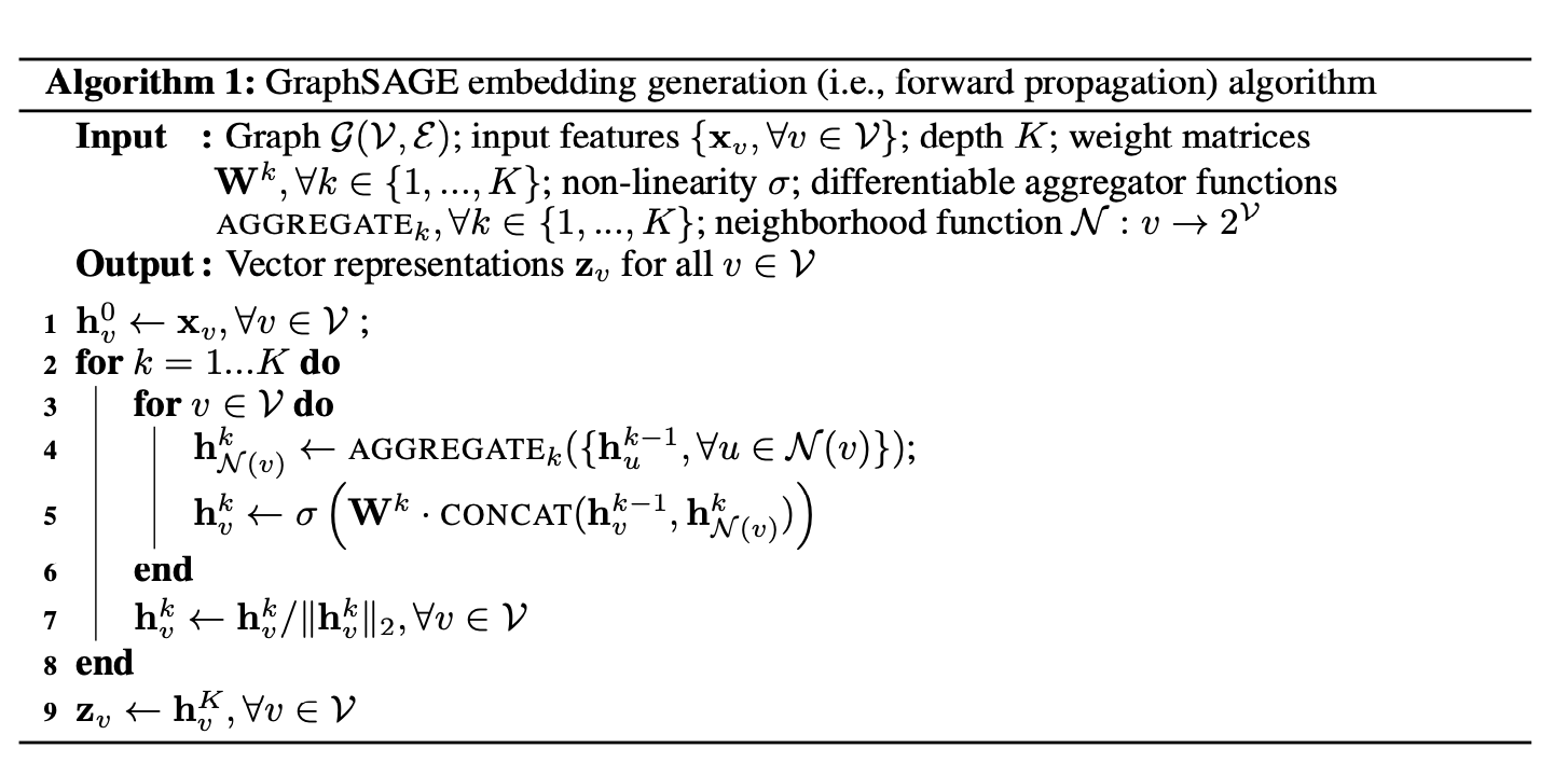
7. GraphSAGE

• Hamilton, Will, Zhitao Ying, and Jure Leskovec. "Inductive representation learning on large graphs." Advances in neural information processing systems 30 (2017).
• GraphSAGE

We now consider the graph convolution from a different aspect. We mimic the logic of convolution on graph: for a 3x3 convolution layer, we conduct weighted average of the value of the 1-step neighbors of the center point. The next layer convolution operation increases the "receptive field" to the 2-step neighbors of the center point.

The algorithm is given below. For each step $k=1, \ldots, K$, we first gather and aggregate all the hidden vecotr from previous step $\mathbf{h}_{u}^{k-1}$ in the neightbourhood of vertex $v$, i.e., $u \in \mathcal{N}(v)$. Then in line 5, we combine the neighborhood information vector $\mathbf{v}_{\mathcal{N}(v)}^k$ with $\mathbf{h}_{v}^{k-1}$ of $v$.

This process has been repeated $K$ times and the information from all the $K$-step neighbor will be included. Instead of training a distinct embedding vector for each node, this algorithm train a set of aggregator functions that learn to aggregate feature information from a node’s local neighborhood.

There are several choices of aggregator function:

• Mean aggregator: which is the average of all the $\left\{\mathbf{h}_{u}^{k-1}, \forall u \in \mathcal{N}(v)\right\}$.

• Pooling aggregator: each neighbor’s vector is independently fed through a fully-connected neural network; following this transformation, an elementwise max-pooling operation is applied to aggregate information across the neighbor set: $$\text { AGGREGATE }_{k}^{\text {pool }}=\max \left(\left\{\sigma\left(W \mathbf{h}_{u}^{k}+\mathbf{b}\right), \forall u \in \mathcal{N}(v)\right\}\right).$$

8. Graph Attention Network

• Veličković, Petar, Guillem Cucurull, Arantxa Casanova, Adriana Romero, Pietro Lio, and Yoshua Bengio. "Graph attention networks." International Conference on Learning Representations (2018).

The input to our layer is a set of node features, $\mathbf{h}=\left\{\vec{h}_{1}, \vec{h}_{2}, \ldots, \vec{h}_{N}\right\}, \vec{h}_{i} \in \mathbb{R}^F$, where $N$ is the number of nodes, and $F$ is the number of features in each node. The layer produces a new set of node features (of potentially different cardinality $F^{\prime}$ ), $\mathbf{h}^{\prime}=\left\{\vec{h}_{1}^{\prime}, \vec{h}_{2}^{\prime}, \ldots, \vec{h}_{N}^{\prime}\right\}, \vec{h}_{i}^{\prime} \in \mathbb{R}^{F^{\prime}}$, as its output.

Consider a self-attention mechanism on the nodes $$e_{i j}=a\left(W \vec{h}_{i}, W \vec{h}_{j}\right),$$ where $W \in \mathbb{R}^{F^\prime \times F}$ is the weight matrix and $a$ is the attention mechanism $a: \mathbb{R}^{F^{\prime}} \times \mathbb{R}^{F^{\prime}} \rightarrow \mathbb{R}$.

Consider the masked attention softmax, which normalize $e_{ij}$ across all the neighbors of node $i$, $$\alpha_{i j}=\operatorname{softmax}_{j}\left(e_{i j}\right)=\frac{\exp \left(e_{i j}\right)}{\sum_{k \in \mathcal{N}_{i}} \exp \left(e_{i k}\right)}.$$ We consider the attention mechanism $a$ as a single-layer feed-forward neural network, parametrized by a weight vector $\overrightarrow{\mathbf{a}} \in \mathbb{R}^{2 F^{\prime}}$, and applying the LeakyReLU non-linearity, $$\alpha_{i j}=\frac{\exp \left(\operatorname{LeakyReLU}\left(\overrightarrow{\mathbf{a}}^{T}\left[W \vec{h}_{i} \| W \vec{h}_{j}\right]\right)\right)}{\sum_{k \in \mathcal{N}_{i}} \exp \left(\operatorname{LeakyReLU}\left(\overrightarrow{\mathbf{a}}^{T}\left[W \vec{h}_{i} \| W \vec{h}_{k}\right]\right)\right)}.$$ where $\|$ is the concatenation operation. Therefore, the one-layer graph attention is computed as follows, $$\vec{h}_{i}^{\prime}=\sigma\left(\sum_{j \in \mathcal{N}_{i}} \alpha_{i j} W \vec{h}_{j}\right).$$ Utilizing the multi-head attention mechanism, we can extend the network structure to $$\vec{h}_{i}^{\prime}=\|_{k=1}^{K} \sigma\left(\sum_{j \in \mathcal{N}_{i}} \alpha_{i j}^{k} W^{k} \vec{h}_{j}\right),$$ where $\|$ represents concatenation, $\alpha_{i j}^{k}$ are normalized attention coefficients computed by the $k$-th attention mechanism $\left(a^{k}\right)$, and $W^{k}$ is the corresponding input linear transformation's weight matrix. Note that, in this setting, the final returned output, $\vec{h}_i^{\prime} \in \mathbb{R}^{K F^{\prime}}$.